Iron Powder Example
This example demonstrates how to use nbragg to analyze neutron transmission through an iron powder sample.
Dataset Overview
The iron powder example showcases the analysis of Bragg edges in a polycrystalline iron sample. We’ll walk through the entire process from data loading to fitting and interpretation.
Data Preparation
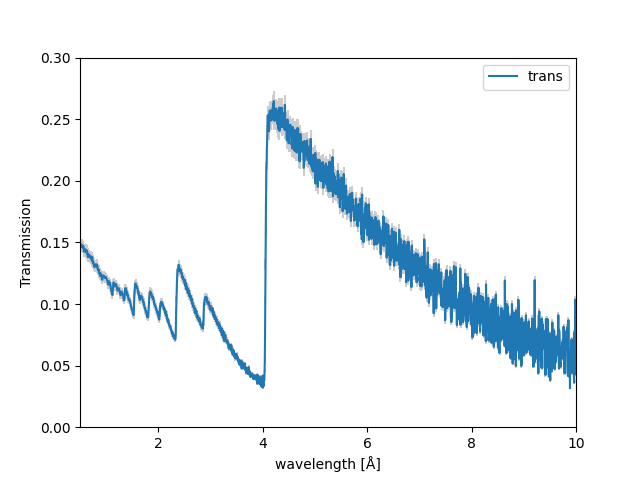
First, load the transmission data and use the .plot method to plot and inspect the data.
import nbragg

# Load transmission data
data = nbragg.Data.from_transmission("iron_powder.csv")
data.plot()
The user can also inspect the data in a table format by calling:
data.table
wavelength |
trans |
err |
|
|---|---|---|---|
0 |
0.501098 |
0.148315 |
0.004449 |
1 |
0.505493 |
0.147728 |
0.004432 |
2 |
0.509889 |
0.147725 |
0.004432 |
3 |
0.514284 |
0.148043 |
0.004441 |
4 |
0.518680 |
0.148369 |
0.004451 |
Cross-Section Configuration
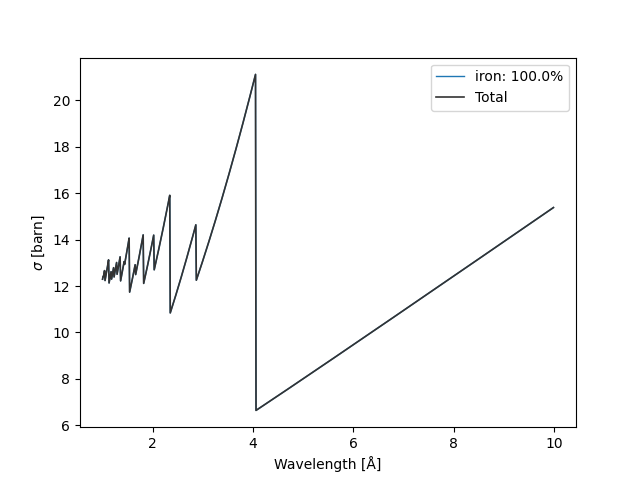
We’ll use the NCrystal cross-section for alpha-iron and use the .plot method to visualize the cross-section:
# Define iron cross-section
xs = nbragg.CrossSection.from_material("Fe_sg229_Iron-alpha.ncmat")
xs.plot()
Model Creation and Fitting
Create a transmission model with background and response variations:
# Create transmission model
model = nbragg.TransmissionModel(
    xs,
    vary_background=True,
    vary_response=True
)

# Perform fitting
result = model.fit(data)
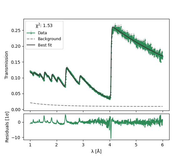
Visualization
Display the fit results using the command:
result.plot()
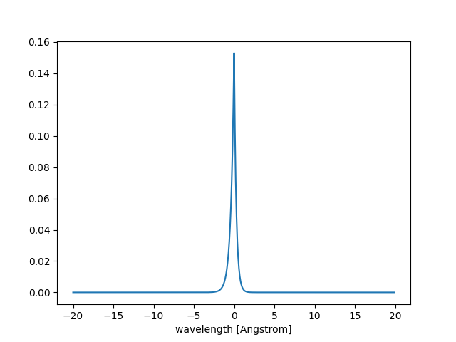
To visualize the instrumental response after fitting, use:
model.response.plot(params=result.params)
Fit Summary
In a Jupyter Notebook, typing result displays the following fit summary as an interactive HTML table:
Fit Result
Model: Model(transmission)
Fit Statistics
Fitting Method |
leastsq |
# Function Evals |
57 |
# Data Points |
1138 |
# Variables |
7 |
Chi-square |
1728.82713 |
Reduced Chi-square |
1.52858279 |
Akaike Info Criterion |
489.878468 |
Bayesian Info Crit. |
525.137662 |
R-squared |
-345.832688 |
Parameters
Name |
Value |
Standard Error |
Relative Error |
Initial Value |
Min |
Max |
Vary |
|---|---|---|---|---|---|---|---|
thickness |
1.97199144 |
0.02039823 |
(1.03%) |
1.0 |
0.0 |
5.0 |
True |
norm |
0.78300304 |
0.00980444 |
(1.25%) |
1.0 |
0.1 |
10.0 |
True |
temp |
300.000000 |
0.00000000 |
(0.00%) |
300.0 |
77.0 |
1000.0 |
False |
α1 |
2.58192159 |
0.06909434 |
(2.68%) |
3.67 |
0.001 |
1000.0 |
True |
β1 |
3.82826196 |
0.12721525 |
(3.32%) |
3.06 |
0.001 |
1000.0 |
True |
b0 |
-0.0221435 |
0.00722197 |
(32.61%) |
0.0 |
-1e6 |
1e6 |
True |
b1 |
0.00684805 |
0.00222445 |
(32.48%) |
0.0 |
-1e6 |
1e6 |
True |
b2 |
0.03639802 |
0.00512610 |
(14.08%) |
0.0 |
-1e6 |
1e6 |
True |
Correlations
Parameter 1 |
Parameter 2 |
Correlation |
|---|---|---|
b0 |
b1 |
-0.9968 |
thickness |
norm |
+0.9825 |
b0 |
b2 |
-0.9725 |
b1 |
b2 |
+0.9670 |
α1 |
β1 |
+0.6106 |
norm |
b0 |
+0.5964 |
norm |
b1 |
-0.5791 |
thickness |
b0 |
+0.5467 |
thickness |
b1 |
-0.5268 |
norm |
b2 |
-0.4251 |
thickness |
b2 |
-0.3591 |
α1 |
b2 |
+0.1194 |
α1 |
b1 |
+0.1181 |
α1 |
b0 |
-0.1071 |
Key Observations
The iron powder sample shows multiple Bragg edges
Variations in background and instrumental response are accounted for
The model provides insights into material structure
Additional Notes
Ensure you have the correct NCrystal material file
Calibrate your instrumental response carefully
The quality of fitting depends on data resolution